

where

Here, [[omega]] is the vorticity, v is the velocity vector, g is a gravity vector, T is temperature (in density units), [[Omega]] is the angular frequency of the reference frame, k is the thermometric diffusivity, [[upsilon]] is the kinematic viscosity and [[phi]] is the stream function. All variables are functions of x and z only.
There were several assumptions and conditions imposed upon all of the pieces of code I wrote. These assumptions/conditions were imposed to ensure compatibility of the routines with the code for the final model.
First, the boundary conditions for the project dictated the boundary conditions for the individual pieces. In each case, the boundaries in z were forced to be 0, and the boundaries in x were periodic. This means that we assumed that an infinite number of copies of the computational array were strung out in each direction of x. The purpose of this was to allow for a large physical area in which the traveling waves could propagate. It is similar to a slice of finite height, wrapping circularly around the sun.
The grid was defined to be twice as wide as it was high, and this allowed the grid to be treated as 2[[pi]] by [[pi]] array, in appropriate units.
In order to enforce these boundary conditions, and to allow for finite differences to be taken at the boundaries, the program needed to compute cells located outside the actual computational area, called guard cells or ghost cells. This can be accomplished by several methods, and depending on the location of the boundary, the boundary conditions are computed either by using a linear fit or by using a parabolic fit.
For most functions, the function value in the guard cells in the z direction were defined so as to make the value of the function at the boundary located between the top/bottom cell of the actual computation area and the guard cell equal to 0. In other words, the grid line between these two points was made to be zero. This was typically calculated by fitting a parabola to the points, and calculating what the value of the guard cell would need to be in order to force this point to be zero. The formula for these z guard cells in the parabolic fit method is:

where f(1/2) is the value of the boundary condition we want to force the z axis to, in our case 0. For our model, this value was zero, so the equation was slightly simplified.
In the x axis, the job was much simpler. Because the function is periodic, the guard cells in the left guard column should have the same the values as the cells in the last (rightmost) column of the actual function. One can think of the guard cells technically as the last column of the previous copy of the function. Similarly, the guard cells on the right should be the start of the next copy, and thus equal to the first (leftmost) column of the actual function. As such the guard cells in x can simply be determined by copying the opposite column of the "real" data.
The first equation for which I worked on developing a solver was the vorticity-stream function equation:

In this case, [[omega]] was an array of known elements and dimensions, and the code was designed to determine [[phi]]. The method chosen for the solution of this problem was as follows. By performing a Fourier transform on each row (Fourier transform in x), we are left with the equation:

From this, a finite difference operation can be applied for the partial derivative in z, and the result is as follows:

Multiplying through by -([[Delta]]z)^2 and using the equality [[Delta]]x=[[Delta]]y=[[Delta]] results in the following:

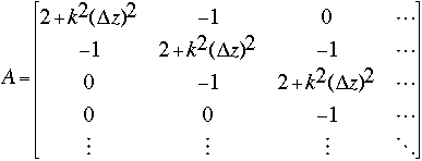
What we then have is nx systems of nz equations in nz unknowns. We then need to solve each system using a tridiagonal matrix solve. A tridiagonal matrix is a matrix in which all the information is contained on the main diagonal and the two diagonals above and below it. This type of matrix is natural for representing finite difference systems, as when a vector is multiplied by this matrix, the j, j-1 and j+1 terms are correctly accounted for. The matrix we required to represent our difference operation is as follows:

We were solving a system of the form Ax=y where A was a matrix and x and y represented vectors. The two vectors represent 'slices' of constant k (columns) from the matrix that represents the Fourier transformed versions of [[omega]] and [[phi]] respectively, and the matrix A represents the differential operator. The Fourier transformed version of [[omega]] was known, as was the differential operation matrix, so the problem was reduced to simply solving for x in the system. This was accomplished using a predefined routine in the ESSL mathematical libraries, and the result was a single Fourier component of [[phi]] as a function of z. When all vectors were determined, nz inverse Fourier transforms were performed, and we had the values of [[phi]] we were looking for. After putting them back together, the original matrix representation for the entire function [[phi]] could be recreated.
The next step in working on the code was the development of a program which would solve the diffusion equation. The general form of the diffusion equation is as follows:

With no source term, the function [[theta]] decays as an exponential of time. By stepping through this frame by frame, the function can be seen to decay from its initial shape to a nearly flat surface. This term is a part of the overall equation which describes the behavior of fluids in general.
The general method of this time-stepping program is to compute the rate of change in temperature, and then compute a new value of the temperature field at each point, based upon the size of the time step and the computed rate of change in temperature there. This prediction is improved upon by several "corrector" steps. After that, an update is performed, and the cycle is repeated.
The next step in the program was to add more terms to the diffusion solver. When this was done, we had code that modeled the following equation:

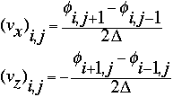
The velocity fields vx and vz were determined from an input stream function [[phi]] to be as follows:

Thus, given the initial temperature field T, the time invariant stream function [[phi]] and the value of the constant R, we have all the variables we need for the system, and can simply advance the system in time and watch the resulting change in the temperature field T. The new term in this differential equation is:

This can be calculated using finite difference methods to be:

With these terms, we subjected to the system to the initial conditions of T=0, [[phi]]=sin x sin z. With these conditions, we expected the temperature field to change in time, and to develop structure. This section worked properly, as the expected structure did, in fact, develop.